Quantifying Arrow Strength

By quantifying the strength of an arrow, we answer the question:

How strong is the causal influence from a cause to its direct effect?

How to use it

To see how the method works, let us generate some data.

>>> import numpy as np, pandas as pd, networkx as nx
>>> from dowhy import gcm
>>> np.random.seed(10)  # to reproduce these results

>>> Z = np.random.normal(loc=0, scale=1, size=1000)
>>> X = 2*Z + np.random.normal(loc=0, scale=1, size=1000)
>>> Y = 3*X + 4*Z + np.random.normal(loc=0, scale=1, size=1000)
>>> data = pd.DataFrame(dict(X=X, Y=Y, Z=Z))

Next, we will model cause-effect relationships as a probabilistic causal model and fit it to the data.

>>> causal_model = gcm.ProbabilisticCausalModel(nx.DiGraph([('Z', 'Y'), ('Z', 'X'), ('X', 'Y')]))
>>> causal_model.set_causal_mechanism('Z', gcm.EmpiricalDistribution())
>>> causal_model.set_causal_mechanism('X', gcm.AdditiveNoiseModel(gcm.ml.create_linear_regressor()))
>>> causal_model.set_causal_mechanism('Y', gcm.AdditiveNoiseModel(gcm.ml.create_linear_regressor()))
>>> gcm.fit(causal_model, data)

Finally, we can estimate the strength of incoming arrows to a node of interest (e.g., \(Y\)).

>>> strength = gcm.arrow_strength(causal_model, 'Y')
>>> strength
    {('X', 'Y'): 41.321925893102716,
     ('Z', 'Y'): 14.736197949517237}

Interpreting the results: By default, the measurement unit of the scalar values for arrow strengths is variance for a continuous real-valued target, and the number of bits for a categorical target. Above, we observe that the direct influence from \(X\) to \(Y\) (~41.32) is stronger (by ~2.7 times) than the direct influence from \(Z\) to \(Y\) (~14.73). Roughly speaking, “removing” the arrow from \(X\) to \(Y\) increases the variance of \(Y\) by ~41.32 units, whereas removing \(Z \to Y\) increases the variance of \(Y\) by ~14.73 units.

In the next section, we explain what “removing” an edge implies. In particular, we briefly explain the science behind our method for quantifying the strength of an arrow.

Understanding the method

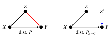
We will use the causal graph below to illustrate the key idea behind our method.

Recall that we can obtain the joint distribution of variables \(P\) from their causal graph via a product of conditional distributions of each variable given its parents. To quantify the strength of an arrow from \(Z\) to \(Y\), we define a new joint distribution \(P_{Z \to Y}\), also called post-cutting distribution, obtained by removing the edge \(Z \to Y\), and then feeding \(Y\) with an i.i.d. copy of \(Z\). The i.i.d. copy can be simulated, in practice, by applying random permutation to samples of \(Z\). The strength of an arrow from \(Z\) to \(Y\), denoted \(C_{Z \to Y}\), is then the distance (e.g., KL divergence) between the post-cutting distribution \(P_{Z \to Y}\) and the original joint distribution \(P\).

\[C_{Z \to Y} := D_{\mathrm{KL}}(P\; || P_{Z \to Y})\]

Note that only the causal mechanism of the target variable (\(P_{Y \mid X, Z}\) in the above example) changes between the original and the post-cutting joint distribution. Therefore, any change in the marginal distribution of the target (obtained by marginalising the joint distribution) is due to the change in the causal mechanism of the target variable. This means, we can also quantify the arrow strength in terms of the change in the property of the marginal distribution (e.g. mean, variance) of the target when we remove an edge.

Measuring arrow strengths in different units

By default, arrow_strength employs KL divergence for measuring the arrow strength for categorical target, and difference in variance for continuous real-valued target. But we can also plug in our choice of measure, using the difference_estimation_func parameter. To measure the arrow strength in terms of the change in the mean, we could define:

>>> def mean_diff(Y_old, Y_new): return np.mean(Y_new) - np.mean(Y_old)

and then estimate the arrow strength:

>>> gcm.arrow_strength(causal_model, 'Y', difference_estimation_func=mean_diff)
    {('X', 'Y'): 0.11898914602350251,
     ('Z', 'Y'): 0.07811542095834415}

This is expected; in our example, the mean value of \(Y\) remains \(0\) regardless of whether we remove an incoming arrow. As such, the strength of incoming arrows to \(Y\) should be negligible.

In summary, arrow strength can be measured in different units (e.g., mean, variance, bits). Therefore, we advise users to pick a meaningful unit—based on data and interpretation—to apply this method in practice.