Demo for the DoWhy causal API

We show a simple example of adding a causal extension to any dataframe.

import dowhy.datasets
import dowhy.api

import numpy as np
import pandas as pd

from statsmodels.api import OLS

data = dowhy.datasets.linear_dataset(beta=5,
        num_common_causes=1,
        num_instruments = 0,
        num_samples=1000,
        treatment_is_binary=True)
df = data['df']
df['y'] = df['y'] + np.random.normal(size=len(df)) # Adding noise to data. Without noise, the variance in Y|X, Z is zero, and mcmc fails.
#data['dot_graph'] = 'digraph { v ->y;X0-> v;X0-> y;}'

treatment= data["treatment_name"][0]
outcome = data["outcome_name"][0]
common_cause = data["common_causes_names"][0]
df

	W0	v0	y
0	0.495676	False	0.114497
1	0.271500	True	6.111279
2	0.405087	True	4.467770
3	1.437909	True	10.856139
4	0.853315	False	5.036457
...	...	...	...
995	0.683802	False	0.712246
996	-0.649195	False	-3.760712
997	1.223760	False	4.286952
998	2.577242	True	11.527125
999	0.762801	True	6.146325

1000 rows × 3 columns

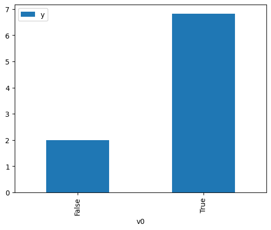
# data['df'] is just a regular pandas.DataFrame
df.causal.do(x=treatment,
                     variable_types={treatment: 'b', outcome: 'c', common_cause: 'c'},
                     outcome=outcome,
                     common_causes=[common_cause],
                     proceed_when_unidentifiable=True).groupby(treatment).mean().plot(y=outcome, kind='bar')

<AxesSubplot: xlabel='v0'>

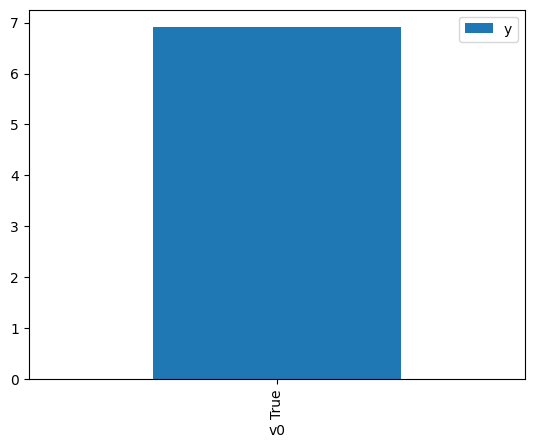
df.causal.do(x={treatment: 1},
              variable_types={treatment:'b', outcome: 'c', common_cause: 'c'},
              outcome=outcome,
              method='weighting',
              common_causes=[common_cause],
              proceed_when_unidentifiable=True).groupby(treatment).mean().plot(y=outcome, kind='bar')

<AxesSubplot: xlabel='v0'>

cdf_1 = df.causal.do(x={treatment: 1},
              variable_types={treatment: 'b', outcome: 'c', common_cause: 'c'},
              outcome=outcome,
              dot_graph=data['dot_graph'],
              proceed_when_unidentifiable=True)

cdf_0 = df.causal.do(x={treatment: 0},
              variable_types={treatment: 'b', outcome: 'c', common_cause: 'c'},
              outcome=outcome,
              dot_graph=data['dot_graph'],
              proceed_when_unidentifiable=True)

cdf_0

	W0	v0	y	propensity_score	weight
0	0.962677	False	2.731163	0.488649	2.046457
1	0.963060	False	1.285152	0.488636	2.046512
2	1.333450	False	2.819011	0.476049	2.100623
3	1.113292	False	4.793211	0.483528	2.068131
4	-0.076380	False	1.492980	0.523985	1.908450
...	...	...	...	...	...
995	0.495474	False	1.407595	0.504545	1.981984
996	0.093358	False	2.586551	0.518220	1.929683
997	-0.649195	False	-3.760712	0.543386	1.840313
998	-0.313608	False	-1.064077	0.532032	1.879586
999	-1.104398	False	-3.100139	0.558712	1.789830

1000 rows × 5 columns

cdf_1

	W0	v0	y	propensity_score	weight
0	1.800934	True	9.604396	0.539792	1.852566
1	0.908676	True	7.848732	0.509514	1.962655
2	1.486907	True	8.214336	0.529158	1.889796
3	2.860181	True	11.082506	0.575341	1.738098
4	0.605184	True	8.075637	0.499188	2.003253
...	...	...	...	...	...
995	0.762801	True	6.146325	0.504551	1.981959
996	-1.252360	True	2.651436	0.436328	2.291852
997	-0.702970	True	1.747041	0.454799	2.198774
998	1.964816	True	8.846990	0.545328	1.833759
999	1.906254	True	6.299404	0.543351	1.840431

1000 rows × 5 columns

Comparing the estimate to Linear Regression

First, estimating the effect using the causal data frame, and the 95% confidence interval.

(cdf_1['y'] - cdf_0['y']).mean()

$\displaystyle 4.70464995857471$

1.96*(cdf_1['y'] - cdf_0['y']).std() / np.sqrt(len(df))

$\displaystyle 0.22224585666512$

Comparing to the estimate from OLS.

model = OLS(np.asarray(df[outcome]), np.asarray(df[[common_cause, treatment]], dtype=np.float64))
result = model.fit()
result.summary()

OLS Regression Results

Dep. Variable:	y	R-squared (uncentered):	0.968
Model:	OLS	Adj. R-squared (uncentered):	0.968
Method:	Least Squares	F-statistic:	1.518e+04
Date:	Mon, 27 Mar 2023	Prob (F-statistic):	0.00
Time:	12:34:22	Log-Likelihood:	-1439.3
No. Observations:	1000	AIC:	2883.
Df Residuals:	998	BIC:	2892.
Df Model:	2
Covariance Type:	nonrobust

	coef	std err	t	P>|t|	[0.025	0.975]
x1	2.3676	0.029	82.056	0.000	2.311	2.424
x2	4.9885	0.052	96.714	0.000	4.887	5.090

Omnibus:	2.708	Durbin-Watson:	1.914
Prob(Omnibus):	0.258	Jarque-Bera (JB):	2.655
Skew:	-0.079	Prob(JB):	0.265
Kurtosis:	3.197	Cond. No.	2.21

Notes:
[1] R² is computed without centering (uncentered) since the model does not contain a constant.
[2] Standard Errors assume that the covariance matrix of the errors is correctly specified.