Conditional Average Treatment Effects (CATE) with DoWhy and EconML
This is an experimental feature where we use EconML methods from DoWhy. Using EconML allows CATE estimation using different methods.
All four steps of causal inference in DoWhy remain the same: model, identify, estimate, and refute. The key difference is that we now call econml methods in the estimation step. There is also a simpler example using linear regression to understand the intuition behind CATE estimators.
All datasets are generated using linear structural equations.
[1]:
%load_ext autoreload
%autoreload 2
[2]:
import numpy as np
import pandas as pd
import logging

import dowhy
from dowhy import CausalModel
import dowhy.datasets

import econml
import warnings
warnings.filterwarnings('ignore')

BETA = 10
[3]:
data = dowhy.datasets.linear_dataset(BETA, num_common_causes=4, num_samples=10000,
                                    num_instruments=2, num_effect_modifiers=2,
                                     num_treatments=1,
                                    treatment_is_binary=False,
                                    num_discrete_common_causes=2,
                                    num_discrete_effect_modifiers=0,
                                    one_hot_encode=False)
df=data['df']
print(df.head())
print("True causal estimate is", data["ate"])
         X0        X1   Z0        Z1        W0        W1 W2 W3         v0  \
0  0.862751  1.748177  1.0  0.374468 -1.404455 -0.675450  2  3  32.691476
1 -1.549036  1.191863  1.0  0.569885 -0.230979  0.694236  0  2  27.991079
2  2.470083  1.181044  1.0  0.935005 -1.283376 -0.529676  3  3  45.170191
3  1.078152 -0.240910  1.0  0.073538 -1.728432  1.071224  2  1  21.107517
4 -0.844955 -0.060493  1.0  0.723959  0.674695 -1.569997  0  0  19.064860

            y
0  606.049152
1  306.567854
2  908.846697
3  253.727307
4  149.472240
True causal estimate is 11.954044739135755
[4]:
model = CausalModel(data=data["df"],
                    treatment=data["treatment_name"], outcome=data["outcome_name"],
                    graph=data["gml_graph"])
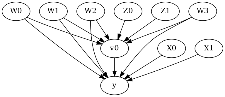
[5]:
model.view_model()
from IPython.display import Image, display
display(Image(filename="causal_model.png"))
[6]:
identified_estimand= model.identify_effect(proceed_when_unidentifiable=True)
print(identified_estimand)
Estimand type: EstimandType.NONPARAMETRIC_ATE

### Estimand : 1
Estimand name: backdoor
Estimand expression:
  d
─────(E[y|W3,W2,W0,W1])
d[v₀]
Estimand assumption 1, Unconfoundedness: If U→{v0} and U→y then P(y|v0,W3,W2,W0,W1,U) = P(y|v0,W3,W2,W0,W1)

### Estimand : 2
Estimand name: iv
Estimand expression:
 ⎡                              -1⎤
 ⎢    d        ⎛    d          ⎞  ⎥
E⎢─────────(y)⋅⎜─────────([v₀])⎟  ⎥
 ⎣d[Z₀  Z₁]    ⎝d[Z₀  Z₁]      ⎠  ⎦
Estimand assumption 1, As-if-random: If U→→y then ¬(U →→{Z0,Z1})
Estimand assumption 2, Exclusion: If we remove {Z0,Z1}→{v0}, then ¬({Z0,Z1}→y)

### Estimand : 3
Estimand name: frontdoor
No such variable(s) found!
Linear Model
First, let us build some intuition using a linear model for estimating CATE. The effect modifiers (that lead to a heterogeneous treatment effect) can be modeled as interaction terms with the treatment. Thus, their value modulates the effect of treatment.
Below the estimated effect of changing treatment from 0 to 1.
[7]:
linear_estimate = model.estimate_effect(identified_estimand,
                                        method_name="backdoor.linear_regression",
                                       control_value=0,
                                       treatment_value=1)
print(linear_estimate)
*** Causal Estimate ***

## Identified estimand
Estimand type: EstimandType.NONPARAMETRIC_ATE

### Estimand : 1
Estimand name: backdoor
Estimand expression:
  d
─────(E[y|W3,W2,W0,W1])
d[v₀]
Estimand assumption 1, Unconfoundedness: If U→{v0} and U→y then P(y|v0,W3,W2,W0,W1,U) = P(y|v0,W3,W2,W0,W1)

## Realized estimand
b: y~v0+W3+W2+W0+W1+v0*X0+v0*X1
Target units: ate

## Estimate
Mean value: 11.954067575947684
EconML methods
We now move to the more advanced methods from the EconML package for estimating CATE.
First, let us look at the double machine learning estimator. Method_name corresponds to the fully qualified name of the class that we want to use. For double ML, it is “econml.dml.DML”.
Target units defines the units over which the causal estimate is to be computed. This can be a lambda function filter on the original dataframe, a new Pandas dataframe, or a string corresponding to the three main kinds of target units (“ate”, “att” and “atc”). Below we show an example of a lambda function.
Method_params are passed directly to EconML. For details on allowed parameters, refer to the EconML documentation.
[8]:
from sklearn.preprocessing import PolynomialFeatures
from sklearn.linear_model import LassoCV
from sklearn.ensemble import GradientBoostingRegressor
dml_estimate = model.estimate_effect(identified_estimand, method_name="backdoor.econml.dml.DML",
                                     control_value = 0,
                                     treatment_value = 1,
                                 target_units = lambda df: df["X0"]>1,  # condition used for CATE
                                 confidence_intervals=False,
                                method_params={"init_params":{'model_y':GradientBoostingRegressor(),
                                                              'model_t': GradientBoostingRegressor(),
                                                              "model_final":LassoCV(fit_intercept=False),
                                                              'featurizer':PolynomialFeatures(degree=1, include_bias=False)},
                                               "fit_params":{}})
print(dml_estimate)
*** Causal Estimate ***

## Identified estimand
Estimand type: EstimandType.NONPARAMETRIC_ATE

### Estimand : 1
Estimand name: backdoor
Estimand expression:
  d
─────(E[y|W3,W2,W0,W1])
d[v₀]
Estimand assumption 1, Unconfoundedness: If U→{v0} and U→y then P(y|v0,W3,W2,W0,W1,U) = P(y|v0,W3,W2,W0,W1)

## Realized estimand
b: y~v0+W3+W2+W0+W1 | X0,X1
Target units: Data subset defined by a function

## Estimate
Mean value: 14.098456720413566
Effect estimates: [[19.90639659]
 [11.58711365]
 [17.30718707]
 ...
 [17.28714141]
 [14.57196521]
 [10.90013775]]
[9]:
print("True causal estimate is", data["ate"])
True causal estimate is 11.954044739135755
[10]:
dml_estimate = model.estimate_effect(identified_estimand, method_name="backdoor.econml.dml.DML",
                                     control_value = 0,
                                     treatment_value = 1,
                                 target_units = 1,  # condition used for CATE
                                 confidence_intervals=False,
                                method_params={"init_params":{'model_y':GradientBoostingRegressor(),
                                                              'model_t': GradientBoostingRegressor(),
                                                              "model_final":LassoCV(fit_intercept=False),
                                                              'featurizer':PolynomialFeatures(degree=1, include_bias=True)},
                                               "fit_params":{}})
print(dml_estimate)
*** Causal Estimate ***

## Identified estimand
Estimand type: EstimandType.NONPARAMETRIC_ATE

### Estimand : 1
Estimand name: backdoor
Estimand expression:
  d
─────(E[y|W3,W2,W0,W1])
d[v₀]
Estimand assumption 1, Unconfoundedness: If U→{v0} and U→y then P(y|v0,W3,W2,W0,W1,U) = P(y|v0,W3,W2,W0,W1)

## Realized estimand
b: y~v0+W3+W2+W0+W1 | X0,X1
Target units:

## Estimate
Mean value: 11.928106208296683
Effect estimates: [[18.16442068]
 [10.44950427]
 [19.96223367]
 ...
 [17.31482748]
 [14.61471155]
 [10.94499818]]
CATE Object and Confidence Intervals
EconML provides its own methods to compute confidence intervals. Using BootstrapInference in the example below.
[11]:
from sklearn.preprocessing import PolynomialFeatures
from sklearn.linear_model import LassoCV
from sklearn.ensemble import GradientBoostingRegressor
from econml.inference import BootstrapInference
dml_estimate = model.estimate_effect(identified_estimand,
                                     method_name="backdoor.econml.dml.DML",
                                     target_units = "ate",
                                     confidence_intervals=True,
                                     method_params={"init_params":{'model_y':GradientBoostingRegressor(),
                                                              'model_t': GradientBoostingRegressor(),
                                                              "model_final": LassoCV(fit_intercept=False),
                                                              'featurizer':PolynomialFeatures(degree=1, include_bias=True)},
                                               "fit_params":{
                                                               'inference': BootstrapInference(n_bootstrap_samples=100, n_jobs=-1),
                                                            }
                                              })
print(dml_estimate)
*** Causal Estimate ***

## Identified estimand
Estimand type: EstimandType.NONPARAMETRIC_ATE

### Estimand : 1
Estimand name: backdoor
Estimand expression:
  d
─────(E[y|W3,W2,W0,W1])
d[v₀]
Estimand assumption 1, Unconfoundedness: If U→{v0} and U→y then P(y|v0,W3,W2,W0,W1,U) = P(y|v0,W3,W2,W0,W1)

## Realized estimand
b: y~v0+W3+W2+W0+W1 | X0,X1
Target units: ate

## Estimate
Mean value: 11.943197314516015
Effect estimates: [[18.1880682 ]
 [10.33805453]
 [20.07307869]
 ...
 [17.39148732]
 [14.69456336]
 [11.0132299 ]]
95.0% confidence interval: [[[18.35894564 10.05480946 20.36054021 ... 17.62456349 14.8707081
   11.08048539]]

 [[18.80908922 10.58132886 20.90920616 ... 18.01789526 15.20684261
   11.41113906]]]
Can provide a new inputs as target units and estimate CATE on them.
[12]:
test_cols= data['effect_modifier_names'] # only need effect modifiers' values
test_arr = [np.random.uniform(0,1, 10) for _ in range(len(test_cols))] # all variables are sampled uniformly, sample of 10
test_df = pd.DataFrame(np.array(test_arr).transpose(), columns=test_cols)
dml_estimate = model.estimate_effect(identified_estimand,
                                     method_name="backdoor.econml.dml.DML",
                                     target_units = test_df,
                                     confidence_intervals=False,
                                     method_params={"init_params":{'model_y':GradientBoostingRegressor(),
                                                              'model_t': GradientBoostingRegressor(),
                                                              "model_final":LassoCV(),
                                                              'featurizer':PolynomialFeatures(degree=1, include_bias=True)},
                                               "fit_params":{}
                                              })
print(dml_estimate.cate_estimates)
[[14.31908135]
 [11.88836565]
 [11.63947806]
 [12.02321801]
 [11.82570109]
 [12.91615893]
 [12.67964213]
 [12.61267616]
 [13.95881387]
 [12.58137557]]
Can also retrieve the raw EconML estimator object for any further operations
[13]:
print(dml_estimate._estimator_object)
<econml.dml.dml.DML object at 0x7f5069843af0>
Works with any EconML method
In addition to double machine learning, below we example analyses using orthogonal forests, DRLearner (bug to fix), and neural network-based instrumental variables.
Binary treatment, Binary outcome
[14]:
data_binary = dowhy.datasets.linear_dataset(BETA, num_common_causes=4, num_samples=10000,
                                    num_instruments=2, num_effect_modifiers=2,
                                    treatment_is_binary=True, outcome_is_binary=True)
# convert boolean values to {0,1} numeric
data_binary['df'].v0 = data_binary['df'].v0.astype(int)
data_binary['df'].y = data_binary['df'].y.astype(int)
print(data_binary['df'])

model_binary = CausalModel(data=data_binary["df"],
                    treatment=data_binary["treatment_name"], outcome=data_binary["outcome_name"],
                    graph=data_binary["gml_graph"])
identified_estimand_binary = model_binary.identify_effect(proceed_when_unidentifiable=True)
            X0        X1   Z0        Z1        W0        W1        W2  \
0    -0.310723  1.922655  0.0  0.181429 -0.253389 -1.406705 -0.268338
1    -0.007636 -0.192476  0.0  0.398953  0.646262  2.191962 -0.390390
2    -0.794449  0.239381  0.0  0.575185  0.177764 -0.279108  1.662390
3    -0.565284 -0.717913  0.0  0.509630 -1.016201  2.030037 -0.697991
4     1.106224  0.331832  0.0  0.914166  0.050561  1.340177 -0.610466
...        ...       ...  ...       ...       ...       ...       ...
9995 -0.831373 -0.743833  0.0  0.769729 -0.278298  0.665073 -0.102795
9996 -1.165620  0.463491  0.0  0.388988 -0.755041 -1.840307 -0.121092
9997  0.349217 -0.316695  0.0  0.807472  0.153194  1.494588  0.053944
9998  0.149037 -0.758180  0.0  0.352517  0.383930  1.684649  0.118264
9999 -0.951185  0.407753  0.0  0.369129 -0.962299 -1.665691  0.169371

            W3  v0  y
0    -1.681963   0  0
1     0.018392   1  1
2    -1.276546   1  1
3    -1.280092   1  1
4     1.914911   1  1
...        ...  .. ..
9995 -0.949982   1  1
9996 -0.175266   0  0
9997 -1.606913   1  1
9998 -0.533962   1  1
9999 -1.091016   0  0

[10000 rows x 10 columns]
Using DRLearner estimator
[15]:
from sklearn.linear_model import LogisticRegressionCV
#todo needs binary y
drlearner_estimate = model_binary.estimate_effect(identified_estimand_binary,
                                method_name="backdoor.econml.dr.LinearDRLearner",
                                confidence_intervals=False,
                                method_params={"init_params":{
                                                    'model_propensity': LogisticRegressionCV(cv=3, solver='lbfgs', multi_class='auto')
                                                    },
                                               "fit_params":{}
                                              })
print(drlearner_estimate)
print("True causal estimate is", data_binary["ate"])
*** Causal Estimate ***

## Identified estimand
Estimand type: EstimandType.NONPARAMETRIC_ATE

### Estimand : 1
Estimand name: backdoor
Estimand expression:
  d
─────(E[y|W3,W2,W0,W1])
d[v₀]
Estimand assumption 1, Unconfoundedness: If U→{v0} and U→y then P(y|v0,W3,W2,W0,W1,U) = P(y|v0,W3,W2,W0,W1)

## Realized estimand
b: y~v0+W3+W2+W0+W1 | X0,X1
Target units: ate

## Estimate
Mean value: 0.5879468116939096
Effect estimates: [[0.64225875]
 [0.5877716 ]
 [0.57993331]
 ...
 [0.59344082]
 [0.57517659]
 [0.58080179]]

True causal estimate is 0.4092
Instrumental Variable Method
[16]:
import keras
dims_zx = len(model.get_instruments())+len(model.get_effect_modifiers())
dims_tx = len(model._treatment)+len(model.get_effect_modifiers())
treatment_model = keras.Sequential([keras.layers.Dense(128, activation='relu', input_shape=(dims_zx,)), # sum of dims of Z and X
                                    keras.layers.Dropout(0.17),
                                    keras.layers.Dense(64, activation='relu'),
                                    keras.layers.Dropout(0.17),
                                    keras.layers.Dense(32, activation='relu'),
                                    keras.layers.Dropout(0.17)])
response_model = keras.Sequential([keras.layers.Dense(128, activation='relu', input_shape=(dims_tx,)), # sum of dims of T and X
                                    keras.layers.Dropout(0.17),
                                    keras.layers.Dense(64, activation='relu'),
                                    keras.layers.Dropout(0.17),
                                    keras.layers.Dense(32, activation='relu'),
                                    keras.layers.Dropout(0.17),
                                    keras.layers.Dense(1)])

deepiv_estimate = model.estimate_effect(identified_estimand,
                                        method_name="iv.econml.iv.nnet.DeepIV",
                                        target_units = lambda df: df["X0"]>-1,
                                        confidence_intervals=False,
                                method_params={"init_params":{'n_components': 10, # Number of gaussians in the mixture density networks
                                                              'm': lambda z, x: treatment_model(keras.layers.concatenate([z, x])), # Treatment model,
                                                              "h": lambda t, x: response_model(keras.layers.concatenate([t, x])), # Response model
                                                              'n_samples': 1, # Number of samples used to estimate the response
                                                              'first_stage_options': {'epochs':25},
                                                              'second_stage_options': {'epochs':25}
                                                             },
                                               "fit_params":{}})
print(deepiv_estimate)
2023-03-27 12:27:16.899280: I tensorflow/core/platform/cpu_feature_guard.cc:193] This TensorFlow binary is optimized with oneAPI Deep Neural Network Library (oneDNN) to use the following CPU instructions in performance-critical operations:  AVX2 AVX512F FMA
To enable them in other operations, rebuild TensorFlow with the appropriate compiler flags.
2023-03-27 12:27:17.104562: W tensorflow/compiler/xla/stream_executor/platform/default/dso_loader.cc:64] Could not load dynamic library 'libcudart.so.11.0'; dlerror: libcudart.so.11.0: cannot open shared object file: No such file or directory
2023-03-27 12:27:17.104604: I tensorflow/compiler/xla/stream_executor/cuda/cudart_stub.cc:29] Ignore above cudart dlerror if you do not have a GPU set up on your machine.
2023-03-27 12:27:17.951119: W tensorflow/compiler/xla/stream_executor/platform/default/dso_loader.cc:64] Could not load dynamic library 'libnvinfer.so.7'; dlerror: libnvinfer.so.7: cannot open shared object file: No such file or directory
2023-03-27 12:27:17.951264: W tensorflow/compiler/xla/stream_executor/platform/default/dso_loader.cc:64] Could not load dynamic library 'libnvinfer_plugin.so.7'; dlerror: libnvinfer_plugin.so.7: cannot open shared object file: No such file or directory
2023-03-27 12:27:17.951277: W tensorflow/compiler/tf2tensorrt/utils/py_utils.cc:38] TF-TRT Warning: Cannot dlopen some TensorRT libraries. If you would like to use Nvidia GPU with TensorRT, please make sure the missing libraries mentioned above are installed properly.
2023-03-27 12:27:18.927155: W tensorflow/compiler/xla/stream_executor/platform/default/dso_loader.cc:64] Could not load dynamic library 'libcuda.so.1'; dlerror: libcuda.so.1: cannot open shared object file: No such file or directory
2023-03-27 12:27:18.927199: W tensorflow/compiler/xla/stream_executor/cuda/cuda_driver.cc:265] failed call to cuInit: UNKNOWN ERROR (303)
2023-03-27 12:27:18.927226: I tensorflow/compiler/xla/stream_executor/cuda/cuda_diagnostics.cc:156] kernel driver does not appear to be running on this host (163d99ee23a1): /proc/driver/nvidia/version does not exist
2023-03-27 12:27:18.927866: I tensorflow/core/platform/cpu_feature_guard.cc:193] This TensorFlow binary is optimized with oneAPI Deep Neural Network Library (oneDNN) to use the following CPU instructions in performance-critical operations:  AVX2 AVX512F FMA
To enable them in other operations, rebuild TensorFlow with the appropriate compiler flags.
Epoch 1/25
313/313 [==============================] - 2s 2ms/step - loss: 10.8053
Epoch 2/25
313/313 [==============================] - 1s 2ms/step - loss: 4.1528
Epoch 3/25
313/313 [==============================] - 1s 2ms/step - loss: 3.6783
Epoch 4/25
313/313 [==============================] - 1s 2ms/step - loss: 3.2178
Epoch 5/25
313/313 [==============================] - 1s 2ms/step - loss: 3.1362
Epoch 6/25
313/313 [==============================] - 1s 2ms/step - loss: 3.0685
Epoch 7/25
313/313 [==============================] - 1s 2ms/step - loss: 3.0406
Epoch 8/25
313/313 [==============================] - 1s 2ms/step - loss: 3.0090
Epoch 9/25
313/313 [==============================] - 1s 2ms/step - loss: 2.9779
Epoch 10/25
313/313 [==============================] - 1s 2ms/step - loss: 2.9491
Epoch 11/25
313/313 [==============================] - 1s 2ms/step - loss: 2.9418
Epoch 12/25
313/313 [==============================] - 1s 2ms/step - loss: 2.9257
Epoch 13/25
313/313 [==============================] - 1s 2ms/step - loss: 2.8966
Epoch 14/25
313/313 [==============================] - 1s 2ms/step - loss: 2.8813
Epoch 15/25
313/313 [==============================] - 1s 2ms/step - loss: 2.8763
Epoch 16/25
313/313 [==============================] - 1s 2ms/step - loss: 2.8627
Epoch 17/25
313/313 [==============================] - 1s 2ms/step - loss: 2.8465
Epoch 18/25
313/313 [==============================] - 1s 2ms/step - loss: 2.8219
Epoch 19/25
313/313 [==============================] - 1s 2ms/step - loss: 2.8060
Epoch 20/25
313/313 [==============================] - 1s 2ms/step - loss: 2.8006
Epoch 21/25
313/313 [==============================] - 1s 2ms/step - loss: 2.7960
Epoch 22/25
313/313 [==============================] - 1s 2ms/step - loss: 2.7781
Epoch 23/25
313/313 [==============================] - 1s 2ms/step - loss: 2.7809
Epoch 24/25
313/313 [==============================] - 1s 2ms/step - loss: 2.7775
Epoch 25/25
313/313 [==============================] - 1s 2ms/step - loss: 2.7763
Epoch 1/25
313/313 [==============================] - 2s 2ms/step - loss: 40602.6328
Epoch 2/25
313/313 [==============================] - 1s 2ms/step - loss: 69124.2734
Epoch 3/25
313/313 [==============================] - 1s 2ms/step - loss: 21931.1914
Epoch 4/25
313/313 [==============================] - 1s 2ms/step - loss: 21394.7734
Epoch 5/25
313/313 [==============================] - 1s 2ms/step - loss: 21423.4043
Epoch 6/25
313/313 [==============================] - 1s 2ms/step - loss: 20895.7148
Epoch 7/25
313/313 [==============================] - 1s 2ms/step - loss: 21310.4961
Epoch 8/25
313/313 [==============================] - 1s 2ms/step - loss: 21517.3457
Epoch 9/25
313/313 [==============================] - 1s 2ms/step - loss: 21268.5645
Epoch 10/25
313/313 [==============================] - 1s 2ms/step - loss: 21685.7969
Epoch 11/25
313/313 [==============================] - 1s 2ms/step - loss: 21055.2480
Epoch 12/25
313/313 [==============================] - 1s 2ms/step - loss: 20993.0918
Epoch 13/25
313/313 [==============================] - 1s 2ms/step - loss: 21059.4609
Epoch 14/25
313/313 [==============================] - 1s 2ms/step - loss: 20939.1973
Epoch 15/25
313/313 [==============================] - 1s 2ms/step - loss: 20945.4180
Epoch 16/25
313/313 [==============================] - 1s 2ms/step - loss: 21184.1582
Epoch 17/25
313/313 [==============================] - 1s 2ms/step - loss: 21025.9551
Epoch 18/25
313/313 [==============================] - 1s 2ms/step - loss: 21019.4688
Epoch 19/25
313/313 [==============================] - 1s 2ms/step - loss: 21132.5977
Epoch 20/25
313/313 [==============================] - 1s 2ms/step - loss: 20835.6816
Epoch 21/25
313/313 [==============================] - 1s 2ms/step - loss: 20880.4961
Epoch 22/25
313/313 [==============================] - 1s 2ms/step - loss: 21244.9863
Epoch 23/25
313/313 [==============================] - 1s 2ms/step - loss: 21052.6562
Epoch 24/25
313/313 [==============================] - 1s 2ms/step - loss: 21159.4043
Epoch 25/25
313/313 [==============================] - 1s 2ms/step - loss: 20908.5078
WARNING:tensorflow:
The following Variables were used a Lambda layer's call (lambda_7), but
are not present in its tracked objects:
  <tf.Variable 'dense_3/kernel:0' shape=(3, 128) dtype=float32>
  <tf.Variable 'dense_3/bias:0' shape=(128,) dtype=float32>
  <tf.Variable 'dense_4/kernel:0' shape=(128, 64) dtype=float32>
  <tf.Variable 'dense_4/bias:0' shape=(64,) dtype=float32>
  <tf.Variable 'dense_5/kernel:0' shape=(64, 32) dtype=float32>
  <tf.Variable 'dense_5/bias:0' shape=(32,) dtype=float32>
  <tf.Variable 'dense_6/kernel:0' shape=(32, 1) dtype=float32>
  <tf.Variable 'dense_6/bias:0' shape=(1,) dtype=float32>
It is possible that this is intended behavior, but it is more likely
an omission. This is a strong indication that this layer should be
formulated as a subclassed Layer rather than a Lambda layer.
302/302 [==============================] - 0s 947us/step
302/302 [==============================] - 0s 953us/step
*** Causal Estimate ***

## Identified estimand
Estimand type: EstimandType.NONPARAMETRIC_ATE

### Estimand : 1
Estimand name: iv
Estimand expression:
 ⎡                              -1⎤
 ⎢    d        ⎛    d          ⎞  ⎥
E⎢─────────(y)⋅⎜─────────([v₀])⎟  ⎥
 ⎣d[Z₀  Z₁]    ⎝d[Z₀  Z₁]      ⎠  ⎦
Estimand assumption 1, As-if-random: If U→→y then ¬(U →→{Z0,Z1})
Estimand assumption 2, Exclusion: If we remove {Z0,Z1}→{v0}, then ¬({Z0,Z1}→y)

## Realized estimand
b: y~v0+W3+W2+W0+W1 | X0,X1
Target units: Data subset defined by a function

## Estimate
Mean value: 2.770221471786499
Effect estimates: [[4.764282 ]
 [4.6206665]
 [3.1853485]
 ...
 [3.8526   ]
 [3.4551697]
 [2.9721527]]
Metalearners
[17]:
data_experiment = dowhy.datasets.linear_dataset(BETA, num_common_causes=5, num_samples=10000,
                                    num_instruments=2, num_effect_modifiers=5,
                                    treatment_is_binary=True, outcome_is_binary=False)
# convert boolean values to {0,1} numeric
data_experiment['df'].v0 = data_experiment['df'].v0.astype(int)
print(data_experiment['df'])
model_experiment = CausalModel(data=data_experiment["df"],
                    treatment=data_experiment["treatment_name"], outcome=data_experiment["outcome_name"],
                    graph=data_experiment["gml_graph"])
identified_estimand_experiment = model_experiment.identify_effect(proceed_when_unidentifiable=True)
            X0        X1        X2        X3        X4   Z0        Z1  \
0    -0.548293 -1.354100 -0.485946  0.109169 -0.341531  1.0  0.343272
1    -0.164619 -2.216070 -0.769799  0.678863 -1.214388  0.0  0.516721
2     0.070081  1.634502  0.431575  1.933633 -0.025654  1.0  0.040302
3    -0.155031  0.188619 -1.829747  1.268342 -0.304938  1.0  0.757539
4     0.029522 -1.510861 -1.440304  0.773982  0.748784  1.0  0.317459
...        ...       ...       ...       ...       ...  ...       ...
9995  0.158801  0.138501 -1.279784 -0.677575 -0.335485  0.0  0.103006
9996 -0.072136 -0.812869 -0.656617  0.854289  0.496226  1.0  0.959045
9997  0.477235 -1.443263  1.285202  0.157785 -0.347817  1.0  0.406434
9998  0.092241 -0.708203 -0.289502  1.765794 -0.393236  0.0  0.838444
9999  0.076762  0.268308 -2.233473 -0.660901 -0.166867  0.0  0.034780

            W0        W1        W2        W3        W4  v0          y
0     1.086304 -1.868620 -1.443568 -0.885970 -0.404444   1  -9.630227
1     1.339322  0.018293  0.349018  1.394824  2.492822   1  19.419568
2     0.785731  0.504848 -2.632900  0.386495  1.549502   1  20.902784
3     0.629309 -0.777420 -1.747567 -0.814652  2.258503   1  12.887155
4     1.594691 -2.014913  1.041188 -1.829288  0.624309   1  15.227367
...        ...       ...       ...       ...       ...  ..        ...
9995  2.040898  1.534510 -3.278571 -1.840978  0.700110   1   2.447969
9996  0.741908  0.364558 -1.507896 -0.176869  1.063277   1   9.814881
9997 -0.012991 -0.142013 -0.799581  0.490618 -0.327751   1   0.959987
9998  1.845220 -0.566965  0.054682 -1.443601 -0.353579   1  14.929544
9999  0.791875  1.691328  1.715514 -1.279265  2.249680   1  32.343029

[10000 rows x 14 columns]
[18]:
from sklearn.ensemble import RandomForestRegressor
metalearner_estimate = model_experiment.estimate_effect(identified_estimand_experiment,
                                method_name="backdoor.econml.metalearners.TLearner",
                                confidence_intervals=False,
                                method_params={"init_params":{
                                                    'models': RandomForestRegressor()
                                                    },
                                               "fit_params":{}
                                              })
print(metalearner_estimate)
print("True causal estimate is", data_experiment["ate"])
*** Causal Estimate ***

## Identified estimand
Estimand type: EstimandType.NONPARAMETRIC_ATE

### Estimand : 1
Estimand name: backdoor
Estimand expression:
  d
─────(E[y|W3,W2,W0,W1,W4])
d[v₀]
Estimand assumption 1, Unconfoundedness: If U→{v0} and U→y then P(y|v0,W3,W2,W0,W1,W4,U) = P(y|v0,W3,W2,W0,W1,W4)

## Realized estimand
b: y~v0+X0+X2+X1+X3+X4+W3+W2+W0+W1+W4
Target units: ate

## Estimate
Mean value: 17.89720388822782
Effect estimates: [[ 3.87972932]
 [19.96464   ]
 [35.12739711]
 ...
 [ 8.32610903]
 [16.79460345]
 [27.54171787]]

True causal estimate is 9.131486470504084
Avoiding retraining the estimator
Once an estimator is fitted, it can be reused to estimate effect on different data points. In this case, you can pass fit_estimator=False to estimate_effect. This works for any EconML estimator. We show an example for the T-learner below.
[19]:
# For metalearners, need to provide all the features (except treatmeant and outcome)
metalearner_estimate = model_experiment.estimate_effect(identified_estimand_experiment,
                                method_name="backdoor.econml.metalearners.TLearner",
                                confidence_intervals=False,
                                fit_estimator=False,
                                target_units=data_experiment["df"].drop(["v0","y", "Z0", "Z1"], axis=1)[9995:],
                                method_params={})
print(metalearner_estimate)
print("True causal estimate is", data_experiment["ate"])
*** Causal Estimate ***

## Identified estimand
Estimand type: EstimandType.NONPARAMETRIC_ATE

### Estimand : 1
Estimand name: backdoor
Estimand expression:
  d
─────(E[y|W3,W2,W0,W1,W4])
d[v₀]
Estimand assumption 1, Unconfoundedness: If U→{v0} and U→y then P(y|v0,W3,W2,W0,W1,W4,U) = P(y|v0,W3,W2,W0,W1,W4)

## Realized estimand
b: y~v0+X0+X2+X1+X3+X4+W3+W2+W0+W1+W4
Target units: Data subset provided as a data frame

## Estimate
Mean value: 14.256874595695916
Effect estimates: [[ 3.1598125 ]
 [17.68565822]
 [22.38831143]
 [10.45220449]
 [17.59838634]]

True causal estimate is 9.131486470504084
Refuting the estimate
Adding a random common cause variable
[20]:
res_random=model.refute_estimate(identified_estimand, dml_estimate, method_name="random_common_cause")
print(res_random)
Refute: Add a random common cause
Estimated effect:12.644451082148896
New effect:12.621608894158342
p value:0.44
Adding an unobserved common cause variable
[21]:
res_unobserved=model.refute_estimate(identified_estimand, dml_estimate, method_name="add_unobserved_common_cause",
                                     confounders_effect_on_treatment="linear", confounders_effect_on_outcome="linear",
                                    effect_strength_on_treatment=0.01, effect_strength_on_outcome=0.02)
print(res_unobserved)
Refute: Add an Unobserved Common Cause
Estimated effect:12.644451082148896
New effect:12.640582788049203
Replacing treatment with a random (placebo) variable
[22]:
res_placebo=model.refute_estimate(identified_estimand, dml_estimate,
        method_name="placebo_treatment_refuter", placebo_type="permute",
        num_simulations=10 # at least 100 is good, setting to 10 for speed
        )
print(res_placebo)
Refute: Use a Placebo Treatment
Estimated effect:12.644451082148896
New effect:0.008593789152544652
p value:0.3694413401817636
Removing a random subset of the data
[23]:
res_subset=model.refute_estimate(identified_estimand, dml_estimate,
        method_name="data_subset_refuter", subset_fraction=0.8,
        num_simulations=10)
print(res_subset)
Refute: Use a subset of data
Estimated effect:12.644451082148896
New effect:12.59188444560931
p value:0.12147673858659258
More refutation methods to come, especially specific to the CATE estimators.